Omid’s Machine Learning tutorial
This Machine Learning tutorial gives an introductory
overview of what Machine Learning is all about.
This document introduces a large number of subfields
of machine learning and is intended for computer science majors who are
considering to specialize themselves in the field of Machine Learning and
Artificial Intelligence.
Index
Omid’s
Machine Learning tutorial
Problems
with using Euclidian distances.
Probably
Approximately Correct (PAC)
Sample
complexity for finite hypothesis spaces
Concept
learning
Imagine that you shall write a program that shall be
able to come up with a hypothesis and draw conclusions from data that it gets
and from these data be able to predict things in the future. This is, in one sentence,
what concept learning is all about.
Or more
specific, a program shall given a certain inductive bias (or in other words a
set of assumptions) be able to learn things from the data it gets. The input to
the program is first of all the bias itself. Normally, this bias is actually
coded in the program itself, and is not passed on as an actual input. More
about the inductive bias later. Second of all, the input to the program is a
few training examples. All training examples must consist of some attributes.
Each attributes can take values from a specific set of values. Together with
these attributes a true or false statement shall be given.
The program
shall be able to come up with a hypothesis that can find out if a certain
statement is true or false by only knowing the attributes. To do this the
program must have a "version space", which is a set of hypothesis
which it think might be correct. This version space is set by the programmer.
He decides the set of all hypotheses. The program never learns anything else
but hypothesis that is in this set, and hence, the program can not learn a
hypothesis that the programmer has not given the computer. The program is only
able to select one or more hypothesis among a set of hypothesis.
The program shall given a train data and a true/false
statement change the size of the version space by adding or removing
hypothesis. Hopefully the program will finally converge to one and only one
hypothesis which it thinks is correct, and hopefully it has found the correct
hypothesis.
Be aware of
that an inductive learning algorithm can at most guarantee that it is able to
classify the training examples correctly. As the program does not know anything
except our training data, we till try to come up with a correct bias that
represents the real model correctly, and we must also make sure that all
training examples are correct. If these two conditions are fulfilled, we know
that we can create an algorithm that can successfully classify examples that
has not yet been seen.
The idea with concept learning is that the program
starts with no knowledge what so ever except the bias (the assumptions it shall
make later on) and that it shall change the hypothesis when it receives a train
data that can help it change the size of the version space.
Some
programs, or algorithms, might only be interested in the most specific
hypothesis possible, whilst other programs might be interested in the largest
hypothesis.
The most specific hypothesis is a hypothesis that tells
us that if a certain instance is consistent with this hypothesis, then the
instance is definitely a true instance. However, if an instance is not
consistent with the largest hypothesis, then we know for sure that it's not a
true instance.
An example of a training input might be "Last
night I ate chicken with curry sauce and I drank red wine. The food tasted
good." Of course, in a computer we represent all these as some fix
attributes and then the answer to the statement. For example:
(Food, Sauce, Drink) : Taste good?
Where Food = Chicken, Beef, Hamburger
Sauce
= Curry sauce, Béarnaise sauce, brown sauce
Drink
= Lemonade, Red wine, White wine
With the statement made above the values should for
example be:
(Chicken, Curry sauce, Red wine) : Yes
The program shall then, given a few training data
(like the one above) be able to predict:
Will a given combination of attributes result in a
true or false statement.
That is, will the food taste good or bad, given a
certain food, sauce and drink.
Obviously the program can't know something we don't
tell it, unless it can do some assumptions. This is where the bias comes in.
The bias is some assumption(s) that the program makes. For example, it might
assume that if you like two different sauces, then you like all sauces that
exist. If you for example like both curry sauce and Béarnaise sauce, you might
also like brown sauce. Of course, this might not be a true assumption, but we
must make some kind of assumptions, or our program will not be able to "learn"
anything.
Important to keep in mind is that if our assumptions
are wrong, that is if we use an invalid bias, then our program will not
guarantee that the results it returns are actually correct.
There are a few different kinds of biases, or
assumptions:
1.) Rote-Learner:
Rote-Learner has no bias at all. This is the, most naive program that actually
doesn't "learn" anything. It only knows what you tell it. If an
instance has already been seen, it returns the classification seen. Otherwise,
if it has not seen the instance then it fails to classify the instance.
2.) Candidate-Elimination:
Candidate-Elimination has a stronger bias than Rote-Learner. CE assumes that
the correct model exists in its version space. It represents the version space
with both its specific and its most general hypothesis.
3.) Find-S:
Find-S has the largest bias. It assumes that no attribute combinations are true
unless it gets training data showing the opposite. Hence, Find-S ignores all
False-statements in the training set as it has already classified all unknown
instances as false instances.
Find-S, obviously, guarantees that it returns the most specific hypothesis.
The most significant disadvantage with these
algorithms is that they are all sensitive to noisy data. One single incorrect
data in enough to make the result of the program incorrect.
Another disadvantage with these algorithms is that we
in many times don't know the bias.
If the bias is too weak, we will result in a
Rote-Learner like algorithm that can not generalize the input given enough. And
hence we need a very large training set. Maybe a much larger set that is
feasible.
If on the other hand the bias is too strong, then our
assumptions might just not be correct. And hence we make generalization beyond what
we are allowed to do - resulting in an incorrect and invalid hypothesis in the
end.
Note that for example the Candidate-Elimination
algorithm is guaranteed to work if it receives correct training data and if the
correct hypothesis is in the version space. But if the bias is too strong and
the correct hypothesis is not in the version space, then the algorithm might
not work at all.
So in practice it's hard creating a useful application
with these algorithms.
One might wonder what training data the user should
give the program.
Or in case we have a program that gives itself
information (by doing some kind of test and then receiving the result of the
test), what information should be given to the program?
Since answers to different questions will decrease the
entropy by different amount, it's obvious that we shall ask a question that
decreases the entropy as much as possible. Or in other words, we shall ask the
question that maximizes the information we gain.
In general, this means that we shall try to create an
instance that satisfies half the hypotheses in the version space.
Decision
Tree Learning
Decision trees is as the name says a tree, where the
nodes of the tree represent attributes and each branch represents a value that
the corresponding attribute might have.
An instance can be classified by walking through the
tree - from the root and down - and for each node, we take the path that
corresponds to the attribute value the instance have.
A decision tree can be written with if-else-statements,
so as one can understand, the tree is a quite simple structure.
Usually we will prefer as short trees as possible.
Short trees are less noisy to inconsistent training data and increase our
chance to find a correct hypothesis, since it should be considered likely that
the hypothesis we search for can be written using a short formula. It's always
easier to find a tree that fits a given set of training data if we are allowed
to use a very large tree, than if we are only allowed to use a small tree. We can
probably find very many different large trees that fit the training data well,
but usually these large trees are less likely to fit new examples. On the other
hand, a short decision tree is hard to find, but if we can find one it's much
more likely that it will be consistent with new examples as it's a more general
hypothesis.
Note that the size of a hypothesis is not necessary
directly proportional to the size of the tree. Two trees representing the same
hypothesis might have very different sizes if the internal representation if
the attributes are different.
One difference between a learning algorithm using a
decision tree and one using an algorithm such as Candidate-Elimination is that
the CE algorithm represents the set of all hypotheses, while a decision tree
only stores one hypothesis. This means that the decision tree can't know how
many other decision trees are consistent with the training data and it can't
come up with an instance that would be able to optimally resolve among these
different hypotheses. This can be done with the CE algorithm, since it knows
all hypotheses that are consistent with the training data.
However, with a decision tree the programmer does not
have to put up a restriction bias and use assumptions about the data which is necessary
for the CE algorithm. The CE algorithm can't learn hypothesis that the
programmer has not given to it at the start, which has the disadvantage that
the programmer must know what bias should be set. As discussed earlier it might
be difficult to set an appropriate bias so that it's neither to weak or neither
to hard.
With a decision tree algorithm like ID3 we use a
preference bias that just states that we prefer shorter trees to longer trees.
And we prefer to have attributes with a high information gain at the top of the
tree.
We however don't have to make assumptions like how the
hypothesis should look like, which is necessary for the CE algorithm.
With this I don't say that in general, all preference
biases are better than all restriction biases - they both have their advantages
and disadvantages. However, in practise a preference bias is more useful since
we can search for our target function in the entire hypothesis space. The
observant reader might use the same argument to say that a restriction bias
could be better since we don’t search the entire hypothesis space, but we can
in advance eliminate hypothesis that we know are incorrect.
It is possible to use an algorithm that combines and
uses both the restriction bias and the preference bias.
A big disadvantage that the Concept Learning
algorithms that I mentioned earlier are that they are very sensitive to invalid
inputs. One single false training data might seriously affect the hypotheses
that we have. Decision trees on the other hand are very robust to noisy data.
Since the algorithm uses the information gain to decide which attributes shall
located closer to the root a few noisy data won't affect these information
gains so much. And we can simply use a termination criterion for the algorithm
that would accept a hypothesis that is not perfect to the set of all training
data.
So far we have made some comparison between the
advantages and disadvantages with decision trees and the algorithms we learned
before. Let’s see how we actually build up a decision tree:
We first calculate which of all attributes that
contains the maximum information gain and we choose this as the rot node. Then
we recursively do the same thing for each child node until we have that each
possible path in the tree leads to a return value for the function the tree
represents, for example true/false.
So what is the information gain and why does the
algorithm look like it does?
Here information gain is the amount of information (in
bits) we get when we know an attribute.
By knowing a certain attribute we can decrease the
hypothesis space and we come closer to the final hypothesis. The best strategy
is to choose a question that halves the space we look into. This way we can
fast reduce the space until we finally only have one element left and we know
that we are done.
The strict definition of information gain is:

where Sv is the set of all examples that
satisfies A(example)=v.
![]() means that v takes all values that attribute A can take.
means that v takes all values that attribute A can take.
Problems with decision trees:
One problem with decision trees is that we can get a
very large tree, and hence a very complex hypothesis that works well with the
training data, but that is not consistent with the real hypothesis and hence
won't work with new examples.
We say that a hypothesis is over fit if there exist
another hypothesis that better satisfies the real examples, while the over
fitted hypothesis better satisfies the training data.
Over fitting will occur if we for example have random noise
in our training data.
It is likely that we can satisfy the training set with
a tree that is large enough, but the probability that the tree satisfies other
large examples is small if the tree is over fitted.
One simple solution to this problem would be to just
stop increasing the tree after a fix size so that it stops growing before it
perfectly satisfies all training data.
This method is a simple method to implement, but in
practice it has been showed that it's better to build a large tree (that is over
fitted) and then post-prune the tree so it's get smaller.
No matter which method we use we must have a method to
see when our tree has reached a size we are satisfied with so that we shall
stop growing the tree. We have several methods to see this:
* The first method, which is also the easiest to
implement and most common method, is to divide the set of examples we have into
two sets. One for training and building the tree, and the other one for
validating the set.
We then just use the validation set to see if our tree
satisfies the validation examples and we can also use these examples to
post-prune the tree.
* The second method is that we use all examples for
training but then with statistical formulas try to see if we can improve the
tree by post-pruning.
* The last method is based on a heuristic called the
minimum description length and uses a technique to measure the complexity for
the tree and the training examples. It halts the growing of the tree when it
has reached a minimum encoding size.
An other problem with the decision tree model is that
we can't use real attribute values. We can go around this by letting the
algorithm during running divide the real values into discrete intervals. This
can be done in many various ways.
We can extend the ID3-algorithm so that it also can
handle with examples with missing attributes or with different costs to
calculate an attribute.
A missing attribute can simply be set to a value by
doing a statistically analysis and "guess" what value is the most
common and probable for this attribute for this example.
To take into account that each node might have a given
cost to calculate we extend the algorithm to not only look at the information
gain we get for a given attribute, but we weight this with the cost of the given
attribute. In this set we do not only prefer short trees, but also trees with
cheap attributes close to the root.
Artificial
Neural Networks
An artificial neural network (ANN) is a network
consisting of very small building blocks that together builds up a network that
can perform very advanced tasks. In one type of ANN, the one we have discussed
in this course, the smallest building blocks are perceptrons.
A perceptron is a function that has 1 and -1 as
outputs (actually, this is not necessarily entirely true, but we can without
loss of generality use perceptrons with an output value in this range) and
takes a finite number of real valued numbers as input.
If a perceptron has n input values, then it stores n+1
weights that it uses to create its output.
The output is defined as:
![]()
where wi = weights i
x0
= constant set to 1 (for convenience reasons)
xi
= input i , i =1, .. , n
sgn(y)
= / 1 if y > 0
\ -1 otherwise
Now we connect a lot of these nodes to a network where
each input signal goes to one or several perceptrons and all perceptron outputs
goes to one or several perceptron inputs.
On or a few of the perceptrons "in the end"
of the network are used as "output perceptrons".
The output of these perceptrons are the networks
output.
Note that, in opposite to the case with the algorithms
we saw under the chapter of Concept learning and Decision trees, the
perceptrons in theory has an infinite hypothesis space.
Each weight that we have can take infinite number of
real values (in theory) and we have also several of these weights, so the
hypothesis space is enormous even in a computer that does not have "real
real values" (but maybe uses 64 bits types to store these "real"
values).
Many times it's however more convenience to have
perceptrons that are continuous. We might then use the sigmoid threshold unit,
which is defined as:

where wi = weight i
x0
= constant set to 1 (for convenience reasons)
xi
= input i , i =1, .. , n
The sigmoid unit is used since it has some very useful
properties.
For example it has a very nice derivate:
![]()
We will see that this very nice property is just what
we want to have when we will create algorithms to find out the target function.
When are ANNs used?
An ANN has many practical applications. Among others
we have applications such as voice and hand writing recognition. The properties
of the problems ANN is good at solving is when we have errors in the training
data or when long training times are allowed. ANNs will learn after receiving
several thousands learning examples, and some mistakes will not cause any
damage to the algorithms.
Also, ANNs can give outputs that are either real
valued or discrete. The actual output is of course real valued, but we can
easily use some kind of threshold value to make it a discrete value. And if we
have several output perceptrons, then our ANN can represent a vector based
function.
The back draw of ANNs is that humans have significant
difficulties to interpret the actual target function that is found. All
information the ANN contains is the weights, and as the weights are just some
real valued variables, a human being can't easily interpret the ANN.
The hypothesis space for ANNs
As the hypothesis space is nothing but the weights in
our network, we can represent all functions that our network can possibly
represent. This means that with even a practical size network we can represent
enormous amount of functions. ANN is a superior way to find a function that we
know very little about. For example, ANNs that can understand handwriting or
that can drive cars on public highways clearly shows how it is possible to find
functions that are completely unknown to the human but that can be found with
an ANN.
The training process
For each training example that we give to the ANN we
must be able to define how good the ANN output was. We can do this in different
ways, one common method is to use the least square method. Without going into
to many technicalities, imagine you are in a space with the weights as axes. We
can calculate the gradient of the error and then change the weights so that we
go in the negative gradient direction (or the steepest descent direction).
For more detailed information about how to minimize a
function without unconstrained, I refer to any book in basic numerical analysis
or a book in optimization. This is beyond the scoop of this course.
In practice we never train one single perceptron, but
we train an entire network. A single network can not represent non-linear
functions. By having a multi layered network we can represent arbitrary
advanced functions. A two layered network can represent any boolean function or
any continues bounded function. A three layered network can represent any
function!
It's quite obvious why a boolean function can be
represented with a 2 layered network. Let’s say we have n bits as input. Let
the first layer contain 2^n different AND-gates, that is all possible AND-gates
that we can have with a n bit input. Only one of these will be true for a given
input. Now let the second layer contain an OR-gate that takes the output of
those AND-gates that corresponds to the input that shall return true. Hence, we
have explained how we can create an arbitrary boolean function that takes a
n-bit as input. And since n is chosen arbitrary, we have explained how to
create an entirely arbitrary boolean function with 2 layers.
An other training algorithm that we use for
multilayered networks is the back propagation algorithm. Now we use the sigmoid
threshold unit!
Also the back propagation algorithm uses a gradient
descent method to find the best hypothesis.
But now we don't train a single perceptron, but we
minimize the total error of the network.
I won't go into details on how the algorithm works,
but in short we have the least square error of all outputs in the space with
all the weights as axes. With the gradient (which we easy can get since we use
Sigmoids threshold unit) we know how to change the weights so that the error
will be minimized.
Unless we don't have a convex hypothesis space (which
we in practice never have) we can't be sure that the minimum we found really is
a global minimum. All we can now is that we might have found a local minimum,
but we don't know in case it is a global minimum.
Problems with ANN
ANN can easily be over fitted for the given training
data. Since we are using a gradient descent method we will eventually find a
local minimum for the training data. However, it is possible that the minimum
we have found corresponds to a function that is very over fitted.
One technique we can use to avoid this is the weight
decay method. The idea of this is that we want to keep the weights small, so
that we can bias learning against complex decision surfaces.
An other method that is more common is that we divide
our examples into one set of training examples and one set of validation examples.
The training set is training the ANN, and the validation set is used to know
when we shall terminate the algorithm. When the error increases for the
validation set it's likely that we have started over fitting the network, and
hence we should quit.
Bayesian
Learning
Bayesian learning is today a very hot topic and has
lately received much attention by media. Mainly, because there have been much
discussions and articles about the use of Bayesian learning algorithms in new
very effective SPAM filters.
Bayesian learning uses probabilities to estimate how
likely or how unlikely a certain event is. For example, how likely is it that
this message with these words is a SPAM letter?
During the training phase each training example can
increase or decrease probabilities for certain events. For example, if the word
Viagra exists in 37% of all SPAM letters but only in 0.03% of all non-spam
letters, then it's likely, but of course not 100% certain, that a letter with
the word Viagra is a SPAM letter.
The algorithms using Bayesian learning will give
different probabilities to different hypothesise. For example, this letter is a
SPAM with the probability of 54%. The program must of course have given rules
for what actions shall be taken given different probabilities. Shall a mail
with a probability of 54% be thrown away or not?
The theory of Bayesian learning might contain
equations that can be very costly to compute. If we however make certain
assumptions, we might significantly reduce the computations needed. One example
of this is the naive Bayesian algorithm, which we will talk about more later
on.
Bayes Theorem
Bayes theorem is, as thought in all basic courses in
statistics and probabilities:
![]()
P(h|D) = the probability for event h, when we know
that event D has occurred
When we shall look at this formula, which of course is
general, we will say that:
h = a certain hypothesis
D = a set of training data.
Of course, Bayes formula yields for all h and D, no
matter what events h and D represents.
In our case, we have the meanings:
P(h|D) = the probability that hypothesis h holds given
that we have received data D.
P(h) = the
probability that hypothesis h is correct.
P(D|h) = the probability that we receive data D given
that hypothesis h holds.
Maximum a posteriori
What we are interested in is to know, what hypothesis
is the most likely one to be true if we receive a certain data. For example,
two hypotheses might be: (1) This letter is a SPAM letter and (2) this letter
is not a SPAM letter. Which of these hypotheses is the most likely one? That
is, which hypothesis h gives the greatest value for P(h|D).
We denote this maximum probable hypothesis:
![]()
hMAP is the function that is the most
likely hypothesis to be valid given data D.
Not that since we can use Bayes theorem we can rewrite
the formula like:
![]()
Most likelihood
We also have a special name for the hypothesis h that
maximizes P(D|h). This h is called the Maximum likelihood hypothesis and is
denoted:
![]()
A brute force algorithm
Given what we know now we can easily create a very
naive brute force algorithm to find the best hypothesis hMAP:
(1) Calculate,
given the training data, all
![]() .
.
(2) Pick
the greatest P(h|D) and we have found the hMAP, which is the
hypothesis that has the greatest probability to be true.
Obviously, this algorithm requires a lot of
computation and since we might have an enormous amount of hypotheses h, it can
really be infeasible to go through all hypotheses to calculate all P(h|D). So
why do we bother about this algorithm?
Well, the algorithm can be used when making analysis
to other concept learning algorithms.
We shall now do a few assumptions and then see what
conclusions we can draw.
Let’s assume that (1) we have a noise free set D with
training data and (2) that we assume that all hypotheses in our hypothesis
space is equally probable and (3) that the target function is in the hypothesis
space. We can then easily use Bayes theorem and conclude that if h is
consistent with D, then we get:

For hypotheses that are not consistent with D, we will
receive:
P(h|D) = 0
Or we can say these two formulas with words:
As all possible hypotheses have the same probability
to be the correct hypothesis, then all hypotheses in the hypothesis space are
MAP-hypotheses.
And if we remember what we did in the earlier
algorithms we talked about under the chapter Concept Learning we can see that
the assumptions we made for their biases are the same as the 3 assumptions we
have made here (noise free D, equally probable hypotheses and target function
exists in hypothesis space).
For example the FIND-S and the Candidate-Elimination
algorithm will both output a MAP-hypothesis, since we have just showed that any
hypothesis consistent with D will be a MAP-hypothesis.
So, even if we did not at all calculating
probabilities at that moment, we have now shown that the hypothesis received is
the most probable hypotheses.
Continuing our analysis with probabilities we can also
show that the maximum likelihood hypothesis is the hypothesis that minimizes
the squared errors between the observed training data and the hypothesis
prediction, given that the errors in our training data has a normal
distribution with mean 0. Note that now we assume that we have error in our
training set (with mean 0). Also be aware of that we assume that we have no
error in each attribute value, but only error in the target value itself.
Assuming errors in the attributes as well requires even more complicated
proofs.
Without going into technicalities, we were able to
show this by setting up the definition for hML and replacing the p(di|h)
term with the formula for a normal distribution and then show that hML
is equal to the hypothesis that minimizes the sum of the square of the error.
Bayes optimal classifier
Bayes optimal classifier tells us which classification
the most probable classification is given an instance and a set of training
data. This means that an algorithm that uses Bayesian optimal classifier
guarantees that the classification it makes has the highest possible
probability to be a correct classification.
The best classification v is denoted as:
![]()
However, this classification can be very costly to
calculate. To calculate the probabilities for all hypotheses for each new
instance can really be infeasible.
We can instead use Gibbs algorithm that instead of
calculating all hypotheses just picks a random hypothesis in H according to the
posterior probability distribution over H. When we shall predict the next
instance x, we use this h that has been picked by random from H.
If certain conditions are fulfilled, then we can prove
that Gibbs algorithm will give a result that is at most twice as bad as Bayes
optimal classifier. And since Gibbs algorithm is indeed a computationally
feasible algorithm, it can be used with great success in several practical
applications.
Naive Bayes Classifier
A sceptical reader might at this point doubt how
useful these different Bayesian algorithms might be since they all seem to
require a great amount of computational power. The fact is that one common
variant of Bayes algorithm is Naive Bayes Classifier. NBC uses an assumption
that allows us to significantly reduce the amount of computation needed and
hence makes the algorithm very useful in many practical applications.
NBC assumes that the attribute values are
conditionally independent. Using this assumption we can rewrite the equation we
have for the best classifier given attributes a1 to an
as:
![]()
Using Bayes Theorem:
![]()
Finally using our assumption that the attributes are
conditionally independent:
![]()
We shall keep in mind that the assumption we make is
in almost all practical situations where this algorithm is implemented a false
assumption. For example, if we have a letter and we want to determine if this
letter is a SPAM mail, then we might use the Naive Bayesian Classifier and say
that each word in the letter corresponds to one attribute and assume that all
words in the letter are independent from each other. This is obviously not
true, since it’s much more likely that the word “Viagra” follows the word
“buy”, than for example “car”. However, in practice it has been showed that
despite our wrong assumption, the algorithm will still produce very good
results.
However, we must remember that when we use this
algorithm despite that our attributes are not conditionally independent, then
we are not guaranteed that the vNB that we have found equals vMAP.
In our derivation above we could only state that vNB equals vMAP
if the attributes are conditionally independent.
We shall end this chapter of Bayesian Learning by
making a comparison between the Naive Bayes Classifier and the other algorithm
we have previously learned. Obviously the greatest difference is that we with
Naive Bayes Classifier do not actually search through a space of possible
hypotheses. We just calculate probabilities for certain events in our training
data, and given these probabilities we can form our hypothesis.
Instance-Based Learning
Unlike the other machine learning techniques we have
shown, instance-based learning does not create a target function from the
training data. Instead we use all training examples and during the
classification phase we have an algorithm that given the training data and the
instance we try to classify the instance.
Hence, we will not create one single target function,
but instead we can see it as we create and use one target function for each
instance we get, and then we throw this target function away.
Obviously this will require a great deal of
computational power at classification time since a (local) target function will
be created and then a classification is made. However, the benefit is that we
can give a much better result since we don’t have a target function that should
be approximated for the global space, but we can create a local target function
that works well and approximates the true hypothesis much better close to the
instance given than a function that would try to approximate the true
hypothesis on the entire space. Hence we get more accuracy to the cost of
calculations that have to be done.
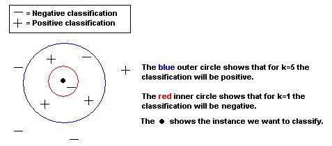
k-Nearest Neighbour learning
The k-Nearest Neighbour learning algorithm takes an
instance and calculates the (Euclidean) distance from the instance that shall be
classified to all training points. Then we consider the k closest training
examples and give the most common classification among these k training
examples. If we have a continuous function we might want to calculate the
average value of these k training examples and return this average value.
If we set k=1 then we will just look for the training
data that is closest to our instance we want to classify, and we classify the
instance with the value the training data has. However, obviously this would be
very sensitive to noise in the training data, so it actually preferred to
instead choose k to a higher value and then give the classification that is the
most common one among these k training examples (or in the continuous case, we
take the average of these k values).
The figure below shows with an example how the
algorithm will work for a problem in 2 dimensions and with 4 positive and 5
negative training examples. The classification for k=1, is false. The
classification for k=5 is true.
How shall we choose the k-value? Shall it be 1, 5 or
100? If it’s too small, noisy data will affect the classification to much, and
if it’s too big many irrelevant training examples will affect the
classification. One solution would be that we give weights to the training
examples we use. A point far away in the space has a low weight and a point
close to the instance has a great weight. We might for example use the weight
formula:
![]()
Where

xq is the instance that shall be classified
and ak(x) is the value of the k:th attribute of instance x.
As we now has an algorithm that actually takes into
account the distance to the points, we might as well take “k=number of training
examples” if we want, since points far away won’t affect the classification
much anyway. However, using many points will of course require much more
computational power, why it is much more practical to set k to a fix and
feasible number. In this way we will have a local search for the best suitable
target function close to the instance and we ignore training examples far away.
Problems with using Euclidian distances
One problem that might arise when we talk about
distances in an n-dimensional space where each dimension represents completely different
attributes (for example weights in kilogram, lengths in meters and times in
milliseconds since 1 January 1970) is that we must have some additional weights
to each attribute.
Lets say that we have an example where each instance
has the following attributes <weight (kilogram), distance (meters), time
elapsed (milliseconds)>. Now we have two training examples and one instance
that we want to classify. The instance we want classify only differs in one
attribute from each training data:
<weight ; distance ; time elapsed>
Instance to classify: <2.8356 ;
42.534 ; 5348536> : ???
Training data 1: <2.8356 ;
42.534 ; 5383351> : true
Training data 2: <3.5716 ;
42.534 ; 5348536> : false
It’s not easy to say if a “distance” of 34815
milliseconds shall be considered greater or less than a “distance” of
By giving different weights we are actually stretching
the coordinate axis so that the points get more spread or closer to the center.
Locally Weighted Regression
Locally Weighted Regression can be seen as a
generalization to the Nearest Neighbour algorithm. As you remember Nearest
Neighbour in some sense created an approximation of the target function in the
point x=xq where xq is the instance we want to classify.
With Locally Weighted regression we however create an approximation to the
target function in a region close to xq. This approximation might be
done in several different ways. We might for example use a linear or a
quadratic function to approximate the target function, or we might even use a
multi layered neural network or any other type of function.
We might for example choose a linear approximation of
the target function such as:
![]()
When we studied the gradient descent method and wanted
to find weights wi to minimize the squared error over a set of
training examples D, then we found the formula:

This later gave us the rule for updating the weights
as follows:
![]()
where h is the learning rate.
(These results were obtained on pages 89-92, Machine
Learning by Tom M. Mitchell, and are derived using the basic gradient descent method.
I have chosen to skip the details of these derivations because I believe the
derivation is not necessary for the reader to continue reading this chapter.)
We can easily modify these results and instead of
minimizing over the entire set of training examples D, we just minimize over
the set of points that are close enough to the point xq:

where Xk,q is the set of the k closest
neighbours of xq.
But remember that we previously said that if we want
we can also minimize over the entire set of D, if we give greater weights to
points close to xq. That leads us to this formula:

Where K(d(xq,x)) is a so called kernel
function that increases when d(xq,x) decreases and vice verse.
So far, we can set K(d(xi,xq))=wi,
but we will soon see more advanced K-functions.
The K-function is as already shown used so we can set
weights to the different attributes depending on how far away they are.
As mentioned once before, it requires a lot of
computational power if we want to go through all training examples, so one
option might be to combine E1 and E2 so we have the
weights, but still only look at the k closest points:

where Xk,q is the set of the k closest
neighbours of xq.
By following the same steps as we did when we derived
the expression for Dwj
in the global minimization case, we can derive an expression for Dwj
from E3 as follows:

where Xk,q is the set of the k closest
neighbours of xq.
Radial basis function
When we try to find a local approximation to the
target function in a point close to xq we might sometimes prefer to
use the radial basis function instead:
![]()
But now we define the kernel function Ku to
be the Gaussian function:

The radial basis approximation approach is actually
both related to the approach by the Locally Weighted Regression with
distance-weights and to the approach by the two-layered artificial neural
network.
The correspondence to the ANN can be seen when we
think of the first layer of the ANN as the values of Ku(d(xu,x))
and the second layer of the ANN where we sum the values of the first layer into
a linear combination.
The advantage of the radial basis function is that we
can train the weights much more effectively than we did in the Local Weighted
Regression case.
There exist many other versions of this method. For
example, we might choose to have k Kernel functions (hidden nodes) – one for
each training example. We center each Gaussian at the point where the
corresponding training example is located (all ss might be
set to the same value). Now we can do a minimization over the entire set of
training examples, but each training example will only influence the value of
f’(x) in a region around x, which is the big advantage of this system. This
also means that later, if we get an instance that is equal to a training
example we know that the approximation will be the same as the real
classification, that is that
![]()
when
![]() .
.
Computational Learning Theory
So far, we have mainly just at some algorithms,
described how they works and in some manner described why the algorithm will work
quite well. However, sometimes why might be interested in actually give
mathematical formulas and bounds to how well our algorithms will work. How many
training examples do we need? What is the probability that the program will
correctly classify a randomly picked instance? How much does the result of the
program if the training data is randomly picked verses if we pick training
examples as we prefer? Etc.
This is what computational learning theory is all
about, to be able to give mathematical formulas to estimate these probabilities
and numbers.
Probably Approximately Correct (PAC)
We shall now consider a model called the probably approximately correct model (or
just the PAC-model), with which we are going to try to find bounds for how many
training examples we must have to be able to with a certain probability get a
program that can correctly classify instances with a certain probability.
But before this, we shall do some restrictions. First
of all, we will only consider noise free training data. Secondly we will only
consider boolean-valued concepts. These assumptions simplify our future
discussions, and the results we receive can still be extended with some
modifications and be used beyond our assumptions.
The problem we are going to consider will be defined
as follows:
- X is as always our set of instances.
- C is the set of target concepts that the learner might want try to
learn.
 is a target
function such
is a target
function such  , where we say that c(x)=1 iff x is a positive example
of x.
, where we say that c(x)=1 iff x is a positive example
of x. is our stationary probability distribution that is used
when we pick a randomly x from X. Note that must be
stationary, that is shall
not change over time.
is our stationary probability distribution that is used
when we pick a randomly x from X. Note that must be
stationary, that is shall
not change over time.- D is the set of training examples.
Note that we are quite general here. We want the
learner to learn an arbitrary ![]() with training examples
taken from an arbitrary distribution
with training examples
taken from an arbitrary distribution ![]() . For this reason we are interested in making worst-case
analysis so that the statements we do shall hold for any
. For this reason we are interested in making worst-case
analysis so that the statements we do shall hold for any ![]() and any distribution
and any distribution ![]() .
.
Errors in hypotheses
There exist two different types of errors that we are
interested in.
One is the error that says how many percent of the
training examples disagrees with our hypothesis h. This is the one that we
relatively easy can obtain as we have the hypothesis h and the training
examples, so we just test and see how many of the examples disagreed to the
hypothesis h. The strict definition is as follows:
![]()
However, the error that we are really interested in
and want to keep as low as possible is the error that says how likely it is that
the hypothesis h misclassifies an x picked with the distribution ![]() from the entire set X.
from the entire set X.
![]()
Although “TrainingErrorD(h)”
might be easy to calculate since we have both h and all training examples, “![]() ” can be really infeasible to calculate since we don’t have
the distribution
” can be really infeasible to calculate since we don’t have
the distribution ![]() .
.
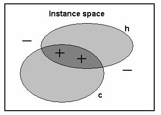
To really understand the great difference between
“TrainingErrorD(h)” and “![]() ” take a look at the figure below. The figure shows a
hypothesis h, at target function c and 4 training examples, 2 positive and 2
negative.
” take a look at the figure below. The figure shows a
hypothesis h, at target function c and 4 training examples, 2 positive and 2
negative.
In this example “TrainingErrorD(h)”
can easily be seen to be 1, since h and c has the same classification on all
training examples. Hence it seems that we have picked a good h. However, as
long as we don’t know anything about the distribution ![]() form which all
instances are picked, we can say nothing about how good h is. Assume that it
shows that the distribution
form which all
instances are picked, we can say nothing about how good h is. Assume that it
shows that the distribution ![]() only picks instances
from the area where h and c disagrees (hence, the training examples are all
“picked” with probability 0%). Then we will make incorrect classification with
probability 100% and correct classification with probability 0%. Suddenly, with
this extra piece of knowledge h doesn’t seem to be as good any longer.
only picks instances
from the area where h and c disagrees (hence, the training examples are all
“picked” with probability 0%). Then we will make incorrect classification with
probability 100% and correct classification with probability 0%. Suddenly, with
this extra piece of knowledge h doesn’t seem to be as good any longer.
PAC learnability
The ideal situation would be if we could make
statements such as “if we pick n training examples we can guarantee that ![]() = 0. However, it’s not possible to make such a strong
assumption. If we want to be absolutely 100% sure that the learner doesn’t
misclassify one single instance x, we must train it with all possible
instances. That is, the training set D must equal the set of possible instances
X. This is of course not feasible in practice. Also, if our training examples
are picked randomly with distribution
= 0. However, it’s not possible to make such a strong
assumption. If we want to be absolutely 100% sure that the learner doesn’t
misclassify one single instance x, we must train it with all possible
instances. That is, the training set D must equal the set of possible instances
X. This is of course not feasible in practice. Also, if our training examples
are picked randomly with distribution ![]() then it’s possible
that we will never pick a certain instance. No matter how many training examples
we pick, we might never get instances with a certain characteristics or
attributes. For example, assume we shall pick 100 randomly chosen values in the
set {0 , 1} with equal probability for zeros and ones. It is possible that we
get 100 zeros and no ones. This is unlikely, but possible.
then it’s possible
that we will never pick a certain instance. No matter how many training examples
we pick, we might never get instances with a certain characteristics or
attributes. For example, assume we shall pick 100 randomly chosen values in the
set {0 , 1} with equal probability for zeros and ones. It is possible that we
get 100 zeros and no ones. This is unlikely, but possible.
So, instead of saying that the ![]() should be zero, we
just say that the error should be less than a given
should be zero, we
just say that the error should be less than a given ![]() . Also, we will weaken the requirement that the
learner must succeed in 100% of the classifications, instead we require that it
shall not fail with a probability higher than
. Also, we will weaken the requirement that the
learner must succeed in 100% of the classifications, instead we require that it
shall not fail with a probability higher than ![]() .
.
Now we have introduced all notations we need to define
what a PAC-learnable concept class C
is:
Def: A concept class C is said to be
PAC-learnable by learner L, using hypothesis H, over the set of instances X of
length n if we have that for all ![]() , X with distribution
, X with distribution ![]() ,
, ![]() and
and ![]() , that learner L will
output a hypothesis
, that learner L will
output a hypothesis ![]() with probability at least (1-
with probability at least (1-![]() ) such that hypothesis
) such that hypothesis ![]() <
< ![]() . This should be done in a time polynomial in
n, size(c), 1/
. This should be done in a time polynomial in
n, size(c), 1/![]() and
1/
and
1/![]() .
.
As the definition of PAC-learnable only considers the
time required for the learner to satisfy the conditions mentioned above, we
must also have a condition on the maximum time for the learner to process each training
example before we can reformulate this to a condition where we give an upper
limit for how many actual training examples are needed before the learner
satisfies the conditions above.
Sample complexity for finite hypothesis spaces
Now we shall look at the sample complexity of problems, which is the growth in required
training examples as the problem size grows. We shall present an upper bound
for ![]() given that the learner
belongs to the class of consistent learners. A consistent learner always
returns hypotheses that have TrainErrorD(h) = 0. That is that the
hypotheses perfectly match the training examples.
given that the learner
belongs to the class of consistent learners. A consistent learner always
returns hypotheses that have TrainErrorD(h) = 0. That is that the
hypotheses perfectly match the training examples.
To do this we will use the version space VSH,D.
As we remember from previous chapters the version space was the set of hypotheses
over H such that the hypotheses perfectly match the training data D. Hence we
know that every consistent learner will output a hypothesis from the version
space. So what we have to do to bound the number of training examples that the
learner needs, we just bound the number of training examples needed to be sure
that the version space contains no hypotheses that does not match the training
examples.
We say that the version space VSH,D. is ![]() -exhausted if all hypotheses in VSH,D.
has an error
-exhausted if all hypotheses in VSH,D.
has an error ![]() <
< ![]() .
.
We can also prove that the probability for that the
version space VSH,D is not ![]() -exhausted is less than
-exhausted is less than ![]() , where 0<
, where 0<![]() <1 and m is the number of independently
randomly drawn training examples from the set D. However, the proof is not
shown here, but can be found at page
<1 and m is the number of independently
randomly drawn training examples from the set D. However, the proof is not
shown here, but can be found at page
Now let’s say that we require that:
![]()
Then we can easily rewrite the above equation to:
![]()
This is indeed a very useful equation, since it tells
us that the number of training examples needed for any consistent learner (no
matter what algorithm is used) to be able to produce a hypothesis h with the
properties mentioned above for ![]() and
and
![]() , grows linearly with respect to 1/
, grows linearly with respect to 1/![]() , and it grows logarithmically with respect to
|H| and 1/
, and it grows logarithmically with respect to
|H| and 1/![]() .
.
Note that all these equations require that H is
bounded in size, so that |H| isn’t infinity. If we want to consider cases where
|H| actually can be infinity, then we must use the Vapnik-Chervonenkis
dimension denoted VC(h).
Agnostic learners
Note that we so far has assumed that we have the
target function c does exists in the hypotheses space that we search through.
That is that we have assumed that the target concept C Î H. However,
sometimes we don’t know if this is the case, and then we want the learner to
find the hypothesis that has the minimum error over the training examples.
Since we might not have a hypothesis that in the
version space that perfectly matches the training data, we want that the error
we have in the best hypothesis should be able to tell us something about the
error for this hypothesis over the entire set of instances with distribution ![]() .
.
It is actually possible to show (although I don’t show
the proof here) that it’s possible to bound the probability that the error over
the entire set of instances shall not be larger than the error for the same
hypothesis over the training example plus a constant ![]() . Or in other words:
. Or in other words:
![]()
Now we make sure that also the worst possible
hypothesis is bounded, so the formula for this becomes:
![]()
This can be rewritten as:
![]()
Note the similarity with the equation be obtained
previously when we assumed that C Î H. Now m grows with the square of 1/![]() , as opposite to the previous equation where it
grew linearly to 1/
, as opposite to the previous equation where it
grew linearly to 1/![]() .
.
Otherwise the equations are equal.
Also, keep in mind that the assumptions we used to get
the first equation were just a special case of the assumptions used now.
Previously we assumed that TrainingErrorD(h)
= 0, so we can rewrite our current inequality as follows:
![]()
Hence, we previously looked at a special case of what we
have now.
Complex Models
When we are talking about Expert Systems we normally
distinguish between the knowledge-base
and the inference-engine. The
knowledge-base is the domain-specific knowledge we have about a certain problem,
whilst the inference-engine is the algorithm(s) that we use to process the data
we have in the knowledge-base. Obviously, both these components are important.
A good database of information is worthless unless we know how we can process
the data and draw reasonable conclusion. However, also the best algorithms will
give useless responses unless they have a good database they can use. That is,
an Expert System requires both a good knowledge-base and an inference-engine.
A Bayesian method
We gone look at an expert system that uses the
Bayesian model.
Assume that we have some different variables that can
be true or false with different probabilities. Assume that given that a certain
variable is true or false, the probabilities for another variable to be true or
false might change. We can then draw this model with a graph structure as the
picture below shows:
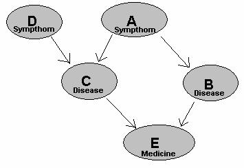
We see that the probability that B is true depends on
A. The probability that C is true depends on both A and D. Finally, the
probability that E is true depends on both B and C.
Now assume that these variables are different medical
conditions or actions a doctor shall take. For example, if a patient has symptom A, then the probability that he
has disease B or C might increase.
However, if a patient has symptom D, then the probability that he has disease C
might increase, but the probability that he has disease B is unaffected. E
might for example mean that the doctor shall give the patient a certain
medicine. Of course, if the patient is likely to have one of the diseases B or
C, the “probability” that the doctor should give medicine E is more likely.
(Actually, it might have been more realistic to have two “Medicine” fields, one
for each disease, but as this is just an example I preferred to keep it small.)
Now let’s say that we have done some studies and found
probabilities for that a patient with certain symptoms have a certain disease
and that a patient with a certain disease should get a certain medicine. Let’s
sat that we know that “if the patient have symptom A, the probability that he
has disease B is X %”. That is, we know have a table with values for all these
probabilities:
P(B | A)
P(B | A’)
P(C | A , D)
P(C | A’ , D)
P(C | A , D’)
P(C | A’ , D’)
P(E | B , C)
P(E | B’ , C)
P(E | B , C’)
P(E | B’ , C’)
(X’ means X is false)
Now we can calculate all probabilities as follows:
![]()


Now, let’s say we have a patient with both symptoms A
and D, what is the probability that we should give this patient medicine E?
That is, what is:
![]()
One obvious way
to solve this is to calculate all 25=32 different
combinations of P(A,B,C,D,E) (when assigning different true/false values to our
5 variables) and then from the value easily calculate P(E,A,D)/P(A,D). We can
easily get P(E,A,D) and P(A,D) by just summing all values from the table that
corresponds to lines where E, A and D are true respectively lines A and D are
true.
The probability for P(A,B,C,D,E) is:
![]()
However, the observant reader can conclude that this
algorithm would indeed be infeasible for greater graphs since the table size is
2n the size grows exponentially with the number of nodes.
Instead we could use a much better algorithm that does
not need to create this entire table, but uses the structure of the graph so it
only calculates a few sums, for example we could calculate P(E,A,D) as follows:
![]()
This of course requires much less computation than
calculating the entire table with all 32 values of P(A,B,C,D,E).
References
- Machine learning by Tom M. Mitchell,
1997.
- Probabilistic Networks
and Expert Systems by Cowell, Dawid, Lauritzen, Spiegelhalter.
- Local computations with
probabilities on Graphical Structures and their Applications to Expert
Systems by S.
L. Lauritzen and D. J. Spiegelhalter, 1988.
- Lectures given by Peter
Damaschke during spring 2004.
- Lectures given by Dag
Wedelin during spring 2004.
Appendix A
Bayesian SPAM Filter
A Bayesian SPAM filter is a program that is supposed
to be able to determine if a given e-mail message is a SPAM message or not. The
filter uses the Naive Bayesian Classifier to classify letters to see if the
letter is a SPAM or not.
The algorithm first needs to train so it learns what a
SPAM message is. So before the filter can be taken into use the user must give
the program a few thousands letters that are classified as SPAM and a few
thousands that are not. If we start train the program with more letters we will
of course get a much more accurate filter, and vice versa. However, a few
thousands letters should be at least a good start.
What the algorithm does is to first create two great
hash tables, one for the SPAM letters and one for the other letters. Each hash
table hashes a word to the number of occurrences of the word in the respective
set of letters. After this is done we create yet another hash that hashes a
word to a probability that the letter in which that word occurs in is a SPAM
message.
Now when we are done with the training we can start
using the filter. For each message we get we go through all words in the mail
and for each word wee see what the chance is that the letter is a SPAM letter.
However, we only consider the most interesting words when we shall make our
final decision if this is a SPAM or not. We might for example consider the top
most interesting 20 words, that is the 20 words that makes it most likely or
unlikely to appear in a SPAM letter. For example words like “Viagra”, “free”
and “color” (you see, spammers love sending HTML messages with different colors
in the text) are likely to appear in SPAM messages, whilst words like “dtek”
(my apartment at the university), “tjena” (the Swedish phrase for “hello”) and
“Omid” (my name) are very unlikely to occur in SPAM letters (but they are very
likely to occur in wanted messages).
So after considering the (for example) 20 most
interesting words we can make a judgement, whether this is a SPAM letter or
not.
Note that when we analyse a mail we both consider not
only the message body, but also the mail headers and HTML-tags in the message.
This will result in that a mail that is sent from one of my classmates with the
e-mail “XYZ@dtek.chalmers.se” will contain the word “dtek” and
“Chalmers”, and hence the message will be very likely to be a non SPAM letter.
However, a SPAM message that contains the “phrase”:
<FONT COLOR=”red”>Buuyy Vi@gr@</FONT>
will have a high probability to be stopped, since both
“red” and “color” are very common in SPAM letters.
We could improve this even more by several different
techniques. For example, we could instead of just considering one single word
at a time consider pairs of words. Then for example the filter would be able to
give a high SPAM probability for “free vacation”, whilst “free software” would
be much less likely to be SPAM.
We could also try to find part of the messages that we
believe are much more interesting than other parts. For example a link to “http://www.naughtygirls.com/”
would be considered as 4 words: “http”, “www”, “naughtygirls” and “com”.
Probably none of these words would make the filter classify this mail as a SPAM
since “http”, “www” and “com” also occurs in non SPAM messages and the word
“naughtygirls” would very likely be a new word that doesn’t already exist in
our database. However, the filter could easily be able to see that “http://www.naughtygirls.com/”
is a link, and we could then try to find separate words in the link. Hence,
“naughtygirls” would become “naughty” and “girls”. Both these would make the
letter get a high probability to be a SPAM letter.
About this document
This document is written by Omid Rouhani ( http://www.OmidRouhani.com/ ).
For contact information, please see ( http://www.OmidRouhani.com/contact.html
).
Copyright 2004-2006; All rights reserved.